
Implementing Integrated Land Use Planning: A step-by-step guide for rural areas
PRACTITIONER’S GUIDE: STEP 5
PART 4
5.1.3. Economic suitability
It is perfectly possible that a physical land evaluation rates a piece of land as highly suitable for one use but marginally suitable for another, yet farmers may still prefer the latter if it leads to higher profit. The idea behind economic land evaluation is that different land utilization types (LUTs) can only be compared using an objective criterion—the monetary value associated with a particular land use.
Economic land evaluation applies general economic principles to compare areas of land under different types of use. This requires estimates of costs and prices, as well as the specification and valuation of capital, labor, and other inputs, alongside yield of produce. Economic land evaluation is particularly useful for setting the boundary between suitability classes S3 and N.
Among the approaches used in land evaluation, gross margin analysis (GMA) and discounted cash flow analysis are the most well-known. Both methods can be easily modeled in a spreadsheet program, enabling the simulation of outcomes based on changes in input variables.
5.1.3.1. Gross margin analysis (GMA)
Gross margin analysis (GMA) is a straightforward method, suitable for analyzing LUTs that involve no capital improvements, only recurring costs and outputs. Its aim is to assess the profitability of a production system from the farmer’s perspective. The analysis begins by breaking down benefits and costs by individual components—such as specific crops or livestock—and then summing these to evaluate the profitability of the entire farming system.
A simplified example of GMA is provided in Box 19.
Box 19. Gross margin analysis: a simplified example
The gross margin is the net income from the sale of produce after production costs and overheads have been subtracted. It can be expressed either per unit area (e.g., per hectare) or per farm/household.
Variable costs include expenditures on seeds, fertilizer, plant protection, machinery, fuel, and labor. These costs are often higher on land with lower physical suitability, for example, due to the need for increased fertilizer use to grow the same crop on sandy soils.
Fixed costs are incurred regardless of whether the land is actually used. These include expenses such as the maintenance of farm buildings, land taxes, and other overhead costs.
Figure 23 presents a theoretical example of a simplified GMA, comparing the economic performance of two crops—wheat and olive—on three land units with differing soil and topographic characteristics.
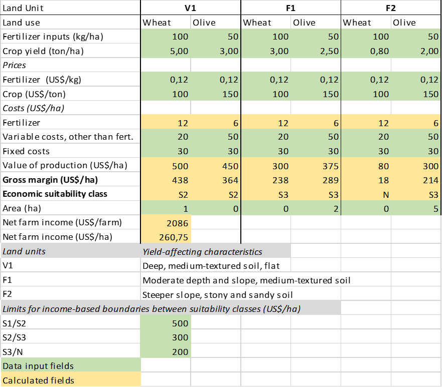
GMA can also be used to define land suitability classes based on economic criteria (i.e., net income). In the example of Figure 23, the limits for the different classes are defined as follows:
- S1 > 500 US$/ha
- S2 = 300–500 US$/ha
- S3 = 200–300 US$/ha
- N ≤ 200 US$/ha
GMA provides a straightforward way to compare how changes in input costs or quantities, produce prices, and yields affect profitability and, consequently, the suitability of land for a particular use.
The feasibility of using GMA depends heavily on the ability to estimate yields on different types of land. This is generally not a problem for individual farmers, and with an adequate sample of representative farm types, GMA has proven effective at local and district levels.
At the national level, however, estimating spatially differentiated yields is one of the most challenging tasks in land evaluation—but it is essential for any economic analysis. Yields at this scale can be estimated through crop modeling (see Section 5.1.1.3) or the Agro-Ecological Zones (AEZ) methodology (Box 13). It is important that these yield estimates are validated by qualified individuals—such as extension officers, farmers, and through statistical surveys.
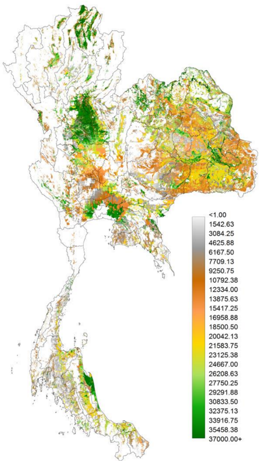
The AEZ methodology also incorporates a generalized economic analysis based on gross margin analysis. Figure 24 illustrates an application of this methodology, in which attainable net revenues were calculated for eight major crops—rice, maize, cassava, soybeans, oil palm, para-rubber, sugarcane, and coffee. This was done using:
• a spatial evaluation of agro-ecologically attainable yields,
• the production cost structure of 2014, and
• average farm gate prices from 2010 to 2014.
In areas where production costs exceeded gross returns (i.e., price × attainable yield), grid cells were marked as economically unsuitable for the respective crop.
5.1.3.2. Discounted cash flow analysis
Discounted cash flow analysis (DCA) is particularly useful when comparing the profitability of LUTs that involve substantial land improvement costs, such as the construction of irrigation infrastructure, afforestation, or the rehabilitation of severely eroded land. In such cases, gross margin analysis (GMA) is inadequate because costs are typically incurred at the start of the project, while benefits accrue over several years.
However, because DCA evaluates the overall economic profitability of large investment projects, it is rarely applied to individual mapping units.
DCA provides a method to compare initial capital expenditures with future benefits, or more generally, to balance costs and benefits that occur at different times in the future. The following key concepts are central to DCA:
- Discount rate (r): the opportunity cost of investing capital in a land improvement project, as opposed to placing it in a savings account or equity investment.
- Net present value (NPV): the theoretical value of all costs and benefits at the start of the project, regardless of when they occur, calculated through discounting.
- Planning horizon: the number of years over which costs are incurred and benefits received.
- Benefit-cost ratio: the present value of benefits divided by the present value of costs.
- Internal rate of return (IRR): the discount rate at which the present value of benefits equals the present value of costs.
A simplified example of DCA is provided in Box 20.
Box 20 Discounted cash flow analysis: a simplified example
Rather than comparing expenditure and benefits at different periods, DCA makes it possible to compare all costs and benefits by taking their present value, through discounting, which is the reverse of compounding interest:
The planning horizon defines how far into the future cash flows (i.e., benefits minus costs) should be projected. In most cases, the period over which it is useful to discount the initial capital investment does not exceed 20 to 30 years.
The benefit-cost ratio (BCR) is a valuable tool for comparing different land uses, particularly when the goal is to maximize return on a limited investment.
If BCR < 1, the land use is economically unsuitable. However, BCR can sometimes be misleading, as low costs and low benefits can result in a high ratio, even if the absolute return is minimal.
The internal rate of return (IRR) represents the interest rate below which a land utilization type (LUT) becomes financially viable. If the prevailing market interest rate is higher than the IRR, the investor would be better off placing their capital in an alternative investment at the going rate rather than proceeding with the project.
Most spreadsheet programs include a built-in function to calculate IRR, making this analysis relatively easy to perform.
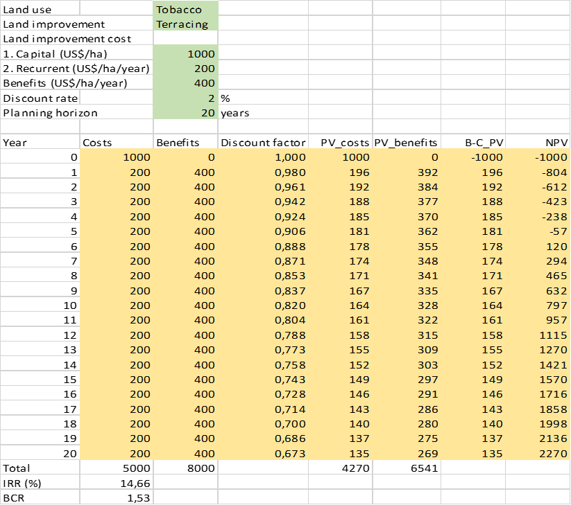
Figure 25 provides a complete calculation demonstrating how costs and benefits incurred at different times can be converted to present value (PV)—that is, adjusted to reflect their value at the start of the project (year 0). In this example, all costs and benefits over a 20-year planning horizon are discounted using a specified discount rate, compressing them into a single time frame for meaningful comparison.
These calculations can be applied to other land utilization types (LUTs), enabling the comparison of their financial attractiveness while accounting for capital expenditures, variable costs, and benefits occurring at different times.
In this example of a cash crop (tobacco) cultivated on steep slopes with newly constructed terraces, the results are as follows:
- Net present value (NPV): 2,270 US$/ha
- Internal rate of return (IRR): 14.7%
- Project lifetime: 20 years
- Nominal discount rate: 2%
Under these conditions—interest rate, benefits, capital and recurrent costs—the investment is economically sound. However, if any of these factors change (e.g., an increase in the discount rate or a decline in expected benefits), the profitability of the project will also be affected.